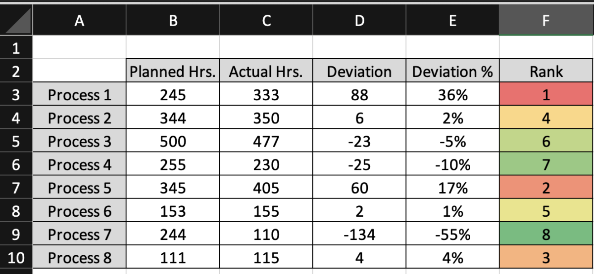
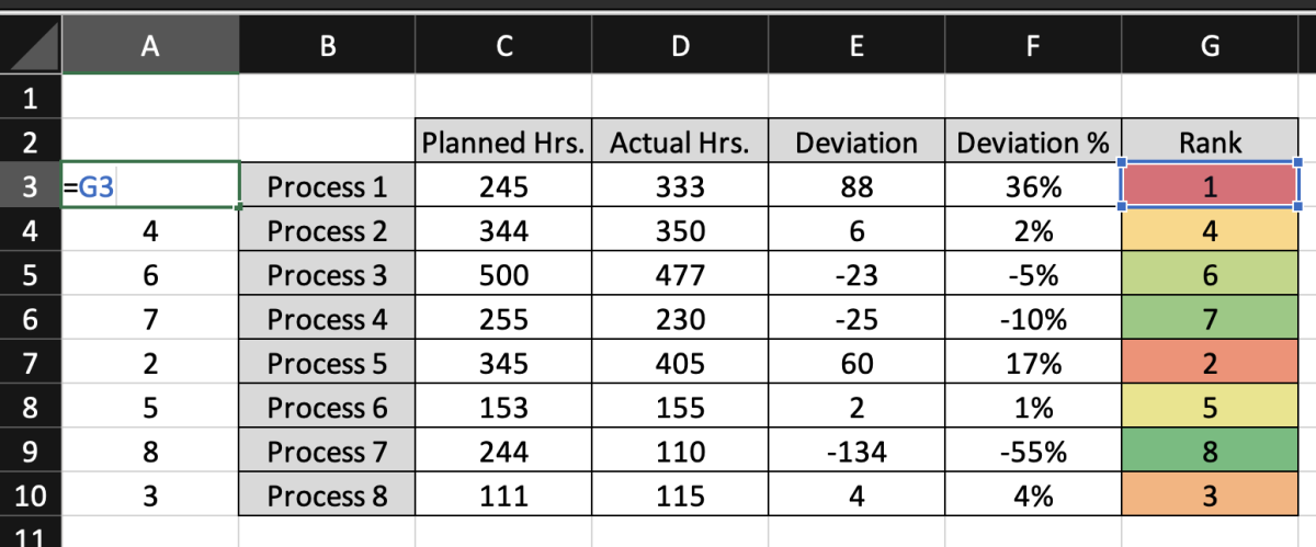
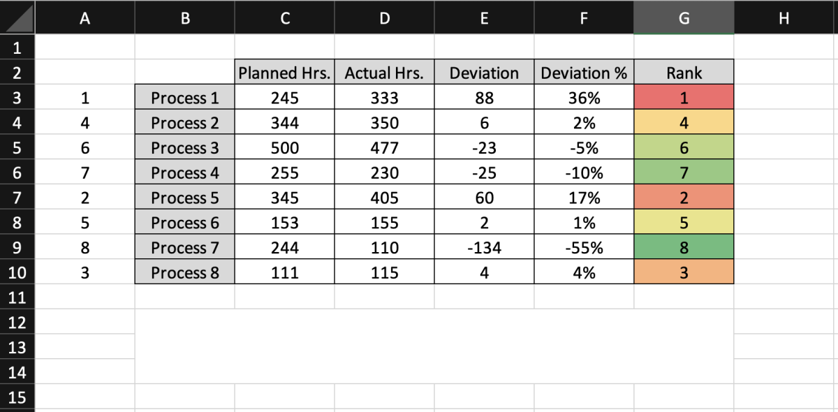
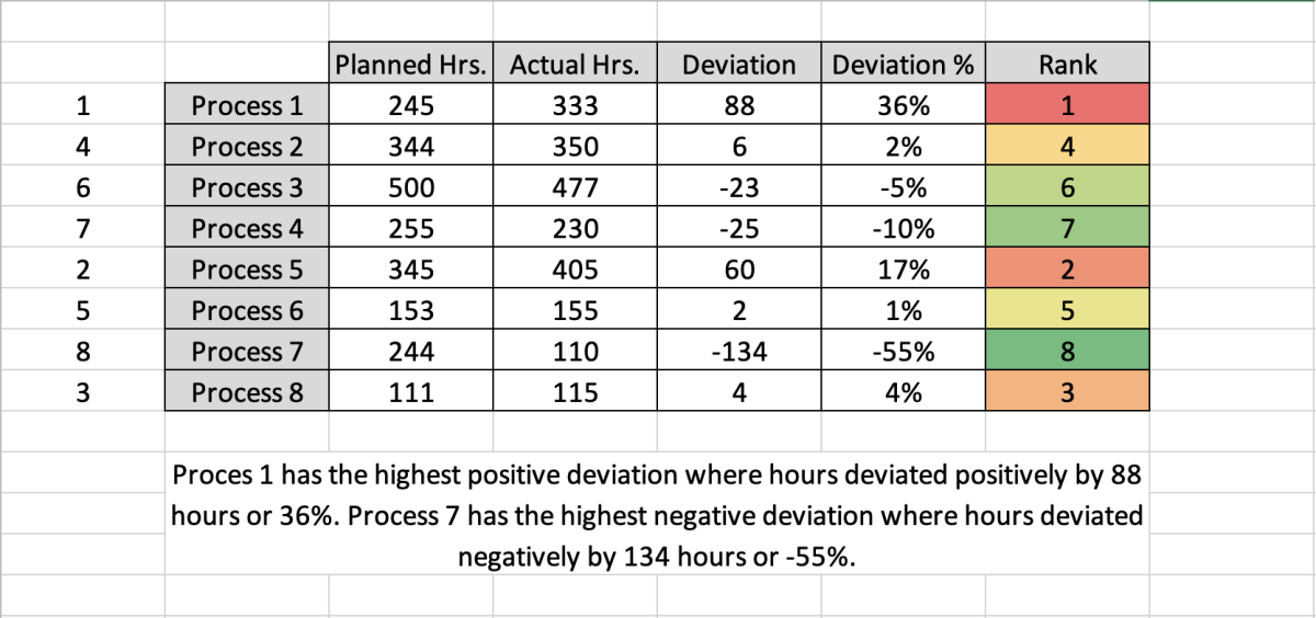
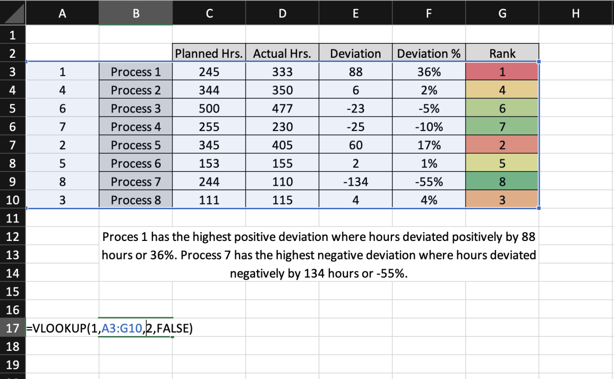
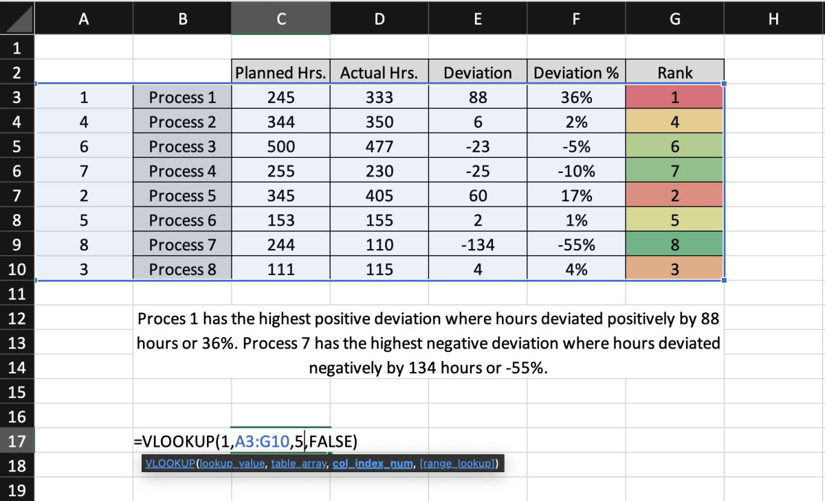
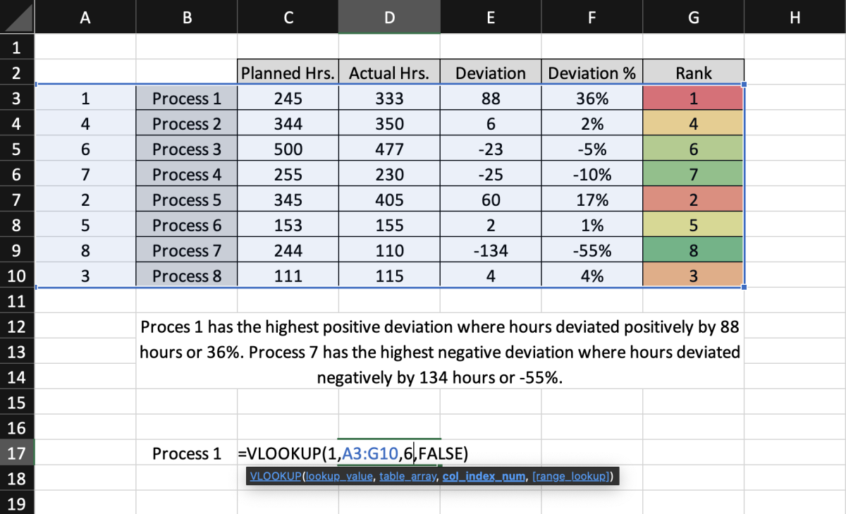
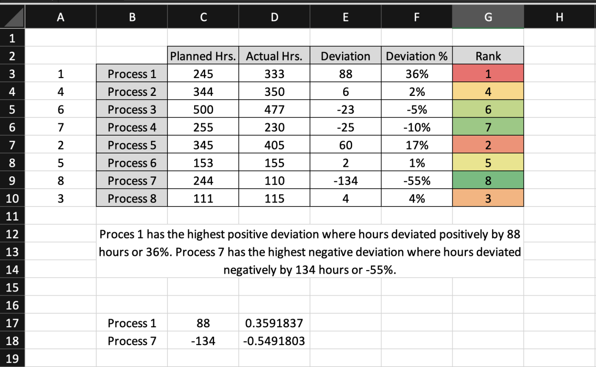
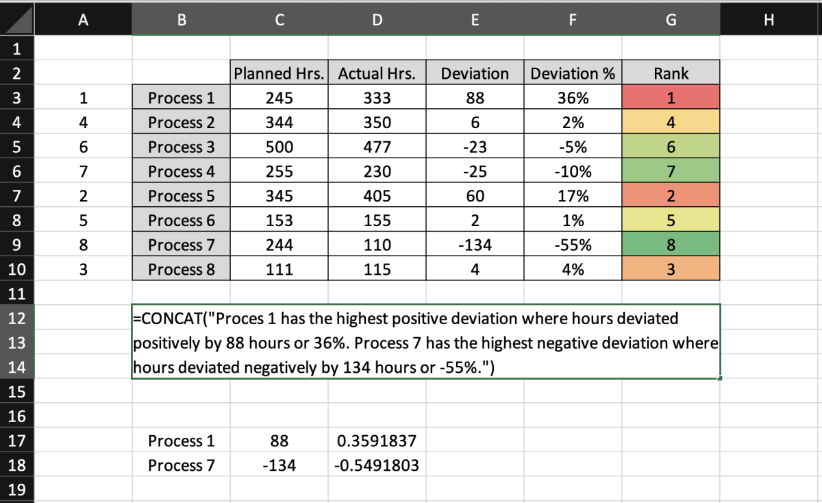
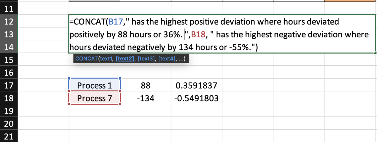
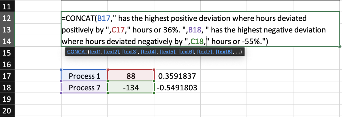
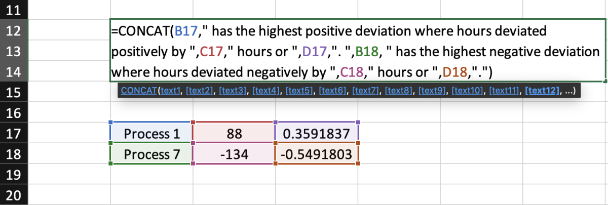
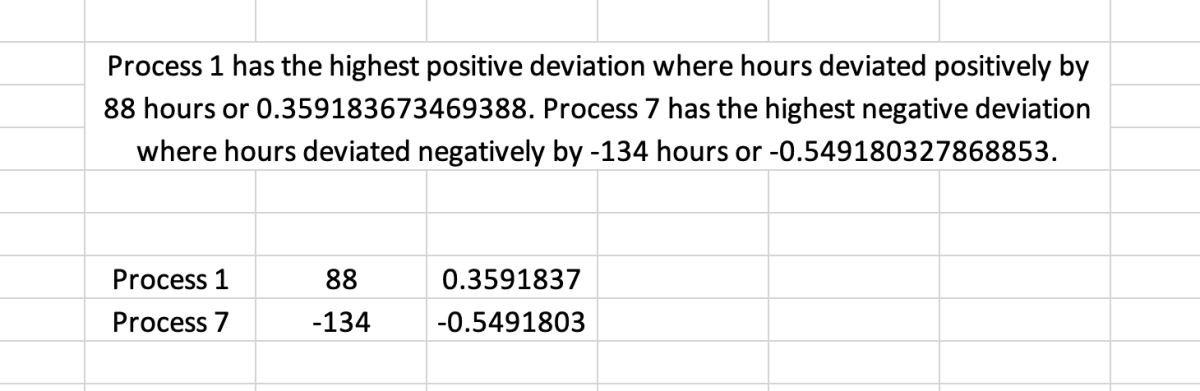
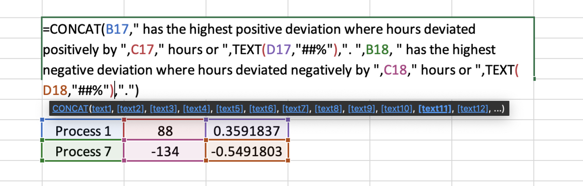
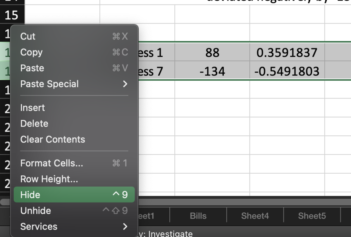
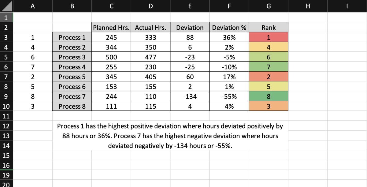
The rank values will determine what value will be pulled into my report so I will first make a dummy column in the first column of the table. Each cell in the dummy column will equal its corresponding rank. See below. I added a new column in front of the table and let the dummy cell for process 1 equal the rank for that process in cell G3. Afterward, I dragged that cell down to repeat the process for each row. Next, I merged and centered an area under the table to hold my report. I also formatted that cell to wrap the text. Now I’m going to create a draft of what I want the report to look like before I create a formula. The draft explains both the highest positive and highest negative deviations of PVA in the data. I will need a formula that pulls the process, deviation, and deviation percent from the table. To decrease the complexity of the formula I use the VLOOKUP function to pull the table data that I need separately. The VLOOKUP function was used below to look up the value in the 1 column and return the process in column 2. To pull the deviation, I essentially copied the same formula to pull the deviation and change the column in the formula to column 5. To pull the deviation percent, I copied the formula over again but used column 6. I used the same formula to pull the highest negative deviation and deviation percentage but used 8 as the lookup value. The next step is to add the CONCAT formula to the report draft, then replace the number with the numbers from the VLOOKUP formulas. I added the CONCAT function to the draft. All text in this formula has to have double quotes around it. Another thing to keep in mind when using the CONCAT formula is that cell values and text can be used but cell values do not need double quotes. Also, a comma needs to be used between every value. In the formula below I replaced Process 1 and Process 7 will cells B17 and B18 respectively. I had to add additional quotes to the formula due to the break in the text. Additionally, a space needs to be added at the beginning and ends of quotes that start or end with a cell reference. Otherwise, the value in the reference and the beginning or end of the text will run together if the space is not accounted for. Next, I replace the deviations with the deviations from the cell references C17 and C18. The percentages in D17 and D18 were also added to the CONCAT function. The TEXT function will need to be used for the percentages. When percent values are concatenated they are changed back to decimals. The TEXT function allows you to format numbers. The first argument in the TEXT function is the value to be formatted and the second argument is the format to be used. The format must have double quotes around it or you will receive an error. Lastly, if you don’t want to look at the cells that contain the VLOOKUP values, you can select those rows and hide them. The great thing about this report is that when the deviations change the report will also update with the new values. This content is accurate and true to the best of the author’s knowledge and is not meant to substitute for formal and individualized advice from a qualified professional. © 2022 Joshua Crowder